

Humble Introduction
First off, thank you for taking time to read this article. I’m writing here not just to summarize my notes and findings, but also to enhance my technical writing skill and sharing what I’ve learned during these few weeks.
A few weeks ago I established an informal research on algorithmic trading and time series data, I decide to start building a crypto trading bot that would retrieve the candlesticks data for every minutes. First I had established the socket connection to Binance Streamer and retrieve real time data successfully, I then continue to build a mathematical algorithm to analyze the movement of k-lines.
As I proceed further, I realized that I was unfamiliar with the concept of arbitrage, Ethereum and smart contract (at least for now), and it really took me a lot of time to do research. Fortunately, I was blessed with great mathematical thinking skills, so modelling mathematical formulae is just a cake walk for me.
Or am I?
Hold on!
Before we start, here are the succinct requirements for building our model.
- Python 3+, or Anaconda installer is preferable.
- Code editors for Python (VScode, Vim, etc.)
- (Optional) IPython/Jupyter notebook for visualization.
- If you aren’t using Ubuntu 22.04, then you need to install python3-tk dependency for matplotlib GUI, installing with
sudo apt install python3-tk.
For me, I’m using Ubuntu 22.04 LTS in Windows 11 WSL 2. I prefer to work with Jupyter notebook inside the VSCode editor and I recommend it for you, too. So you can edit your notebooks and other code files at the same time.
Once you finished setup, continue and install the following Python modules via pip or conda.
- matplotlib
- numpy
- pandas
- scikit-learn
Scientific computing and machine learning are generally heavily rely upon certain packages such as numpy, scipy, matplolib, etc.
Candlestick… Candles? Tick?
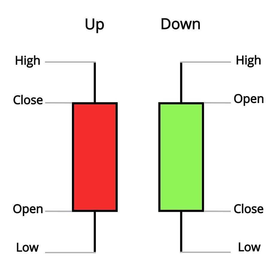
A candlestick (or ticker) is a graphical way of representing the Open, High, Low, Close prices, together with the trades volume. The candlestick commonly abbreviated as OHLCV.
You might saw a candlestick chart before, you may observed that the candles are filled with only two colors: red (bullish) and green (bearish). The bullish candlestick with solid background (or red color) denoted that the close price is higher than the open price, and vice versa for bearish candlestick.
The open and close values correspond to the price of first trade and last trade, respectively.
Gets your hands dirty
It’s time to code now, note that this article is mere technicality and written primarily in Python.
For this article, I cropped out an 1-day BTC-USDT trading data for back-testing. This exported CSV file contained the OHLCV entries for every tick from date 2022/7/15 to 2022/7/16, each tick is with 1-minute interval.
import numpy as np
import pandas as pd
from datetime import datetime

df = pd.read_csv('../data/btcusdt.csv', index_col=False)
df['Opentime'] = pd.to_datetime(df['Opentime'])
del df['Ignore']    # remove unused ignored column

df.info()

# <class 'pandas.core.frame.DataFrame'>
# Int64Index: 2000 entries, 0 to 1999
# Data columns (total 11 columns):
# Column Non-Null Count Dtype
# --- ------------------- --------------   ------------
#	0   Opentime            2000 non-null   datetime64[ns]
#	1   Open                2000 non-null   float64
#	2   High                2000 non-null   float64
#	3   Low                 2000 non-null   float64
#	4   Close               2000 non-null   float64
#	5   Volume              2000 non-null   float64
#	6   Closetime           2000 non-null   int64
#	7   Quote asset volume  2000 non-null   float64
#	8   Number of trades    2000 non-null   int64
#	9   Taker by base       2000 non-null   float64
#	10  Taker buy quote     2000 non-null   float64
# dtypes: datetime64ns, float64(8), int64(2)
# memory usage: 187.5 KB
Compute Log returns
Ultimately, the log-returns are very useful in quantitative finance, especially when you want to do algorithmic trading. Because of its time-additive property, this made our life easier to compute the cumulative returns.
For instance, consider you had collected the close prices over the last 3 minutes.
| Time (minutes) | Close price |
| 1 | 20 |
| 2 | 10 |
| 3 | 25 |
To compute the cumulative sum of log returns, simply summing up all the log prices. Over calculation, all values will get cancelled out, remain only the log returns at time 0 (start) and time n (the last one) as quotient inside log function.

In a generic form, the cumulative log-returns during time interval [0, n] can be formulate as
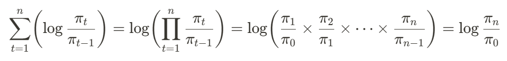
Not only that, the log-value of return is very useful for generating lagged data . But no rush, I will discuss this part later.
When you should back-testing your data?
“Wait a minute, Doc. Are you telling me you built a time machine...out of a DeLorean?”
There are two common approaches for back-testing: Vectorized back-testing and Event-driven back-testing.
Back-testing is about simulate a trading strategy by looking back the historical data. This back-testing strategy aggregate all the related data and transformed them into vectors or arrays and perform linear algebra computation, which are drastically fast. Vectorized back-testing has its limitation, however. It doesn’t means that you can become a billionaire by traveling back in time. The pattern of candlesticks is ephemeral, You can’t just keep changing the parameters just to make it looks nicer during back-testing, this will lead to over-fitting — your model performed well only on historical data but performed poorly on future data.
Another scenario is event-driven back-testing, it provide a higher degree of precision, but the computation cost is much more expensive comparing to the vectorized back-testing approach. The following approach required explicit loops over every bars of the candlesticks data which sacrificed computational speed for higher prediction accuracy.
Predictions on price movement direction
Here’s where it gets serious now.
First we compute the log returns of the underlying asset
df['log_returns'] = np.log(df['Close'] / df['Close'].shift(1))
df.head()
I’ve shifting the original time-series data to reproduce another five lagged versions time-series. The basic idea is that the market prices from last 1-minute and four more minutes back can be used to predict the market price now.
minutes2shift = [1, 2, 3, 4, 5]

def generate_lags(data):
    global cols
    cols = []
    for lag in minutes2shift:
        if 'log_returns' in data:
            col = 'lag_{}'.format(lag)
            data[col] = data['log_returns'].shift(lag)
            cols.append(col)
    print(cols)

generate_lags(df)
df.dropna(inplace=True)
Now transform the lagged values to binary: either 0 or 1.
df[cols] = np.where(df[cols] > 0, 1, 0)and transform the float valued predictions to its sign values: either +1 or -1.
df['direction'] = np.where(df['log_returns'] > 0, 1, -1)Now you can see that the original data table now included the lagged returns and movement directions of log returns. (Note that row 1-5 has been removed since we had dropped all the entries which had contained NaN data type)
df[cols + ['direction']].head()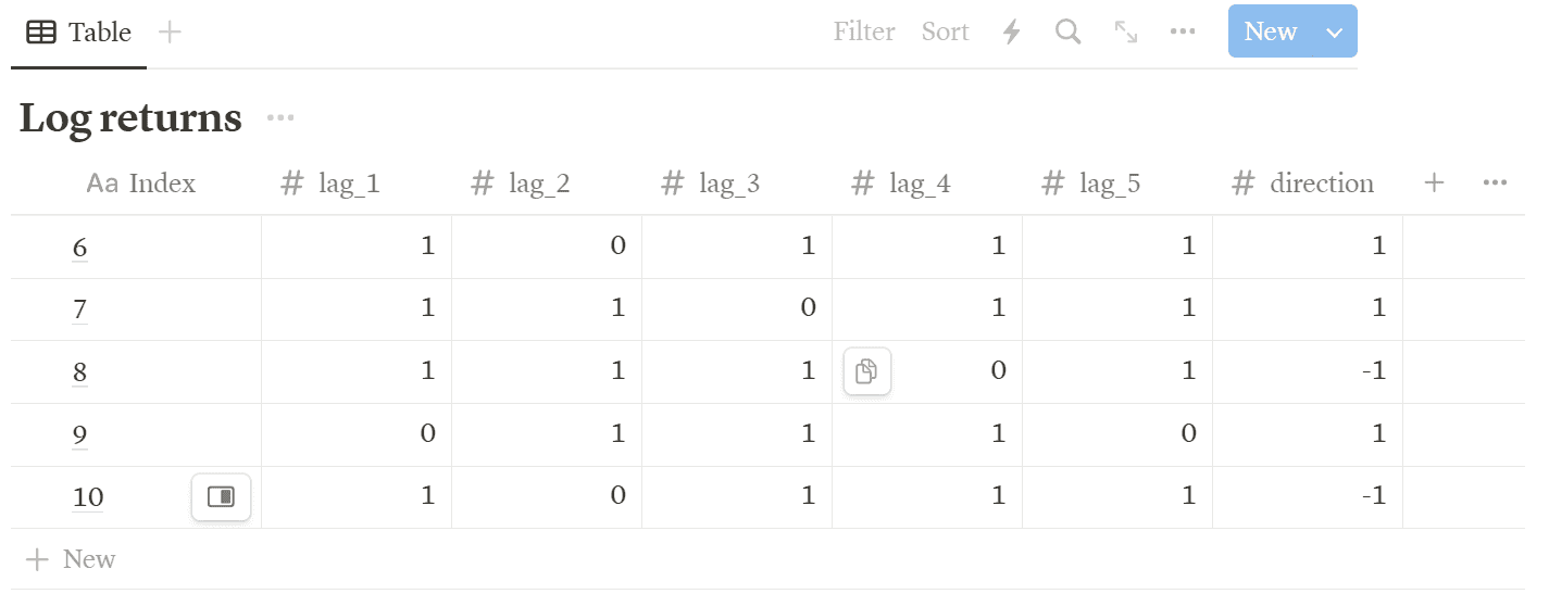
To make prediction on the price movement. You can apply several supervised learning algorithms on our time series. Recall that a supervised learning algorithms are intentionally to perform classification, it required features and label data.
From the tabulated lagged data as shown above, observed that there are only two possible outcomes for direction column: +1 if the price going upward, -1 if the price going downward. Based on the outcomes, I’ve using support vector machine (SVM) to train on 80% of the data frame rows, and testing on the remaining set. The code below trains and tests based on a sequential train-test split.
from sklearn.svm import SVC
from sklearn.metrics import accuracy_score

split = int(len(df) * 0.80)
train = df.iloc[:split].copy()
model = SVC(C=1, kernel='poly', degree=3)
model.fit(train[cols], train['direction'])
At this point, we can now check the accuracy for both training and test data.
test_accuracy = accuracy_score(train['direction'], model.predict(train[cols]))
train_accuracy = accuracy_score(test['direction'], model.predict(test[cols]))
Of course, you can even try using logistic regression for classifying the direction. Because the market directional movement is moving whether upward or downward, as well as labelled with the values +1 and -1. The logistic regression is a binary classifier that performed well on classifying this kind of features data.
from sklearn.linear_model import LogisticRegression

log_reg_model = LogisticRegression().fit(train[cols], train['direction'])
print(accuracy_score(train['direction'], log_reg_model.predict(train[cols])))
This is the accuracy of the predictions from the fitted models:
| SVM with polynomial degree 3 | Logistic Regression | |
| Train (80% of sample) | 0.56050157 | 0.53667711 |
| Test (20% of sample) | 0.52631579 | 0.49624060 |
Despite of logistic regression, I’ll rather choose SVM model. It has a slight edge — in the context of hit ratio. The model which accuracy scores for both test and train data greater than 50% are considered to be good, and our model is better as its accuracy gets closer to one.
Now that we can derive the log returns for the ML-based algorithmic trading strategy, and hence plot our strategy performance.
# derive ML-based strategy
test['strategy'] = test['position'] * test['log_returns']

# Plotting performance of strategy
test[['log_returns', 'strategy']].cumsum() \
    .apply(np.exp) \
    .set_index(test['Opentime']) \
    .plot(figsize=(10, 6))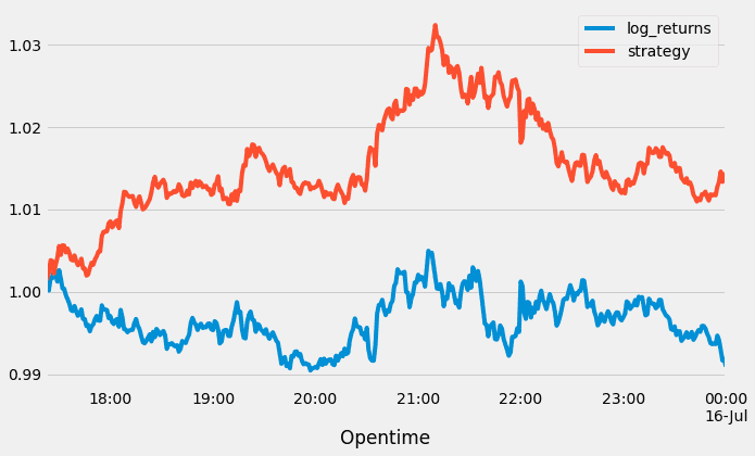
Interpret result with Kelly Criterion
The investing strategy is much likely same as a coin-tossing game, you would gain if your model made a correct guess on the price movement, otherwise you will lose your bets.
Well, as a wise investor, of course we wouldn’t put all your eggs in one basket. So here comes the question: How much fund should we allocate so that the profit can be maximized, and minimize the loss at the same time?
The solution is pretty straight forward. Let me introduce the Kelly criterion— An optimized way to put your bets on a game.
The Kelly criterion is defined as below:
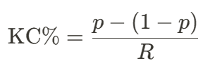
where p is the probability of success, and R is the ratio of the average gain against the ratio of the average loss. Any value of p that’s greater than 0.5 is consider good.
According to Investopedia, however, it recommended that
The percentage (a number less than one) that the equation produces represents the size of the positions you should be taking. For example, if the Kelly percentage is 0.05, then you should take a 5% position in each of the equities in your portfolio. This system, in essence, lets you know how much you should diversify.
For our case, we view our model accuracy score as the probability of success, said p = 0.52. And the odds of win against loss is 1-1, so we have R = 1. Substitute into the formula and calculate will give us the Kelly percentage
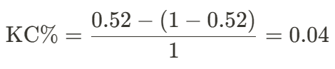
indicating that 4% of your fund can be allocated in BTC-USDT cryptocurrency without worries.
Also, it is recommended to update your optimal fraction after a certain period of time (1 week, 1month, etc.).
Final thoughts
Before I end this post, let’s overview again the full process of vectorized back-testing.
- From the imported time-series data, find the log returns for each timestamp. Note that the log return of 1st row will always be
NaN. - Generates the lagged log returns based on original log returns data. Hence,
- Transform the values from lag 1 to lag 5 to binary data (features).
- Get the sign of log return for each entries (label data).
- Divide your time series data into 80% of training set and 20% of test data. (It depends, you can pick any ratio for training and test).
- Lastly, applying any supervised learning algorithm (OLS Regression, SVM, etc.) to fit your model, with the transformed features and labels as input.
Overall I think this is a good start to build my algorithmic model. However I feel like there are still many things that have not been written.
What’s next?
Thanks for reading, I hope you enjoy reading this post. Feel free to comment below if you have any questions regarding this post. We’re going to learn how to use Deep Neural Network (DNN) model to make prediction on future prices in next topic.
See you then!
References
- J.Kuepper. (2021). Using the Kelly Criterion for Asset Allocation and Money Management. Investopedia. https://www.investopedia.com/articles/trading/04/091504.asp
- Y. Hilpisch. (2019). Python for Finance: Mastering Data-driven Finance (2nd ed.). O’ Reilly